aerocaps.geom.curves.RationalBezierCurve3D#
- class RationalBezierCurve3D(control_points: List[Point3D], weights: ndarray, name: str = 'RationalBezierCurve3D', construction: bool = False)[source]#
Bases:
PCurve3DThree-dimensional rational Bézier curve class
- __init__(control_points: List[Point3D], weights: ndarray, name: str = 'RationalBezierCurve3D', construction: bool = False)[source]#
Creates a three-dimensional rational Bézier curve objects from a list of control points and weights
- Parameters:
control_points (List[Point3D] or numpy.ndarray) – Control points for the Bézier curve
weights (numpy.ndarray) – Weights for the control points. Must have the same length as the control point array
name (str) – Name of the geometric object. May be re-assigned a unique name when added to a
GeometryContainer. Default: ‘RationalBezierCurve3D’construction (bool) – Whether this is a geometry used only for construction of other geometries. If
True, this geometry will not be exported or plotted. Default:False
Methods
compute_t_corresponding_to_x(x_seek[, t0])Computes the \(t\)-value corresponding to a given \(x\)-value
compute_t_corresponding_to_y(y_seek[, t0])Computes the \(t\)-value corresponding to a given \(y\)-value
compute_t_corresponding_to_z(z_seek[, t0])Computes the \(t\)-value corresponding to a given \(z\)-value
d2cdt2(t)Evaluates the second derivative of the curve with respect to \(t\)
dcdt(t)Evaluates the first derivative of the curve with respect to \(t\)
Elevates the degree of the rational Bézier curve.
enforce_c0(other)enforce_c0c1(other)enforce_c0c1c2(other)enforce_g0(other)enforce_g0g1(other, f)enforce_g0g1g2(other, f)evaluate(t)Evaluates the line at one or more \(t\)-values
Evaluates a verbose set of parametric curve data as a class based on an input parameter value or vector
Evaluates the line at one or more \(t\)-values and returns a single point object or list of point objects
generate_from_array(P, weights)get_control_point_array([unit])Gets an array representation of the control points
Gets the array of control points in homogeneous coordinates, \(\mathbf{P}_i \cdot w_i\)
plot(ax[, projection, nt])Plots the curve on a
matplotlib.pyplot.Axesor a pyvista.Plotter windowplot_control_points(ax[, projection])Plots the control points on a
matplotlib.pyplot.Axesreverse()to_iges(*args, **kwargs)Converts the geometric object to an IGES entity.
transform(**transformation_kwargs)Creates a transformed copy of the curve by transforming each of the control points
Attributes
- compute_t_corresponding_to_x(x_seek: float, t0: float = 0.5)[source]#
Computes the \(t\)-value corresponding to a given \(x\)-value
- compute_t_corresponding_to_y(y_seek: float, t0: float = 0.5)[source]#
Computes the \(t\)-value corresponding to a given \(y\)-value
- compute_t_corresponding_to_z(z_seek: float, t0: float = 0.5)[source]#
Computes the \(t\)-value corresponding to a given \(z\)-value
- d2cdt2(t: float) ndarray[source]#
Evaluates the second derivative of the curve with respect to \(t\)
- Parameters:
t (float or int or numpy.ndarray) – Either a single \(t\)-value, a number of evenly spaced \(t\)-values between 0 and 1, or a 1-D array of \(t\)-values
- Returns:
If \(t\) is a
float, the output is a 1-D array containing three elements: the \(x\)- \(y\)-, and \(z\)-components of the second derivative. Otherwise, the output is a 2-D array of size \(\text{len}(t) \times 3\)- Return type:
- dcdt(t: float) ndarray[source]#
Evaluates the first derivative of the curve with respect to \(t\)
- Parameters:
t (float or int or numpy.ndarray) – Either a single \(t\)-value, a number of evenly spaced \(t\)-values between 0 and 1, or a 1-D array of \(t\)-values
- Returns:
If \(t\) is a
float, the output is a 1-D array containing two elements: the \(x\)- \(y\), and \(z\)-components of the first derivative. Otherwise, the output is a 2-D array of size \(\text{len}(t) \times 3\)- Return type:
- elevate_degree() RationalBezierCurve3D[source]#
Elevates the degree of the rational Bézier curve. Uses the same algorithm as degree elevation of a non-rational Bézier curve with a necessary additional step of conversion to/from homogeneous coordinates.
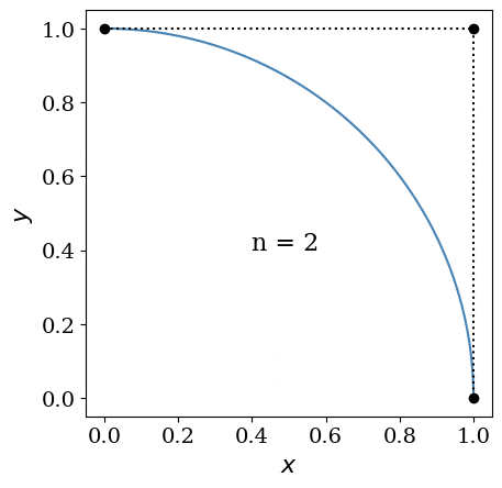
Degree elevation of a quarter circle exactly represented by a rational Bézier curve#
- Returns:
A new rational Bézier curve with identical shape to the current one but with one additional control point.
- Return type:
- evaluate(t: float) ndarray[source]#
Evaluates the line at one or more \(t\)-values
- Parameters:
t (float or int or numpy.ndarray) – Either a single \(t\)-value, a number of evenly spaced \(t\)-values between 0 and 1, or a 1-D array of \(t\)-values
- Returns:
If
tis afloat, the output is a 1-D array with three elements: the values of \(x\), \(y\), and \(x\). Otherwise, the output is an array of size \(\text{len}(t) \times 3\)- Return type:
- evaluate_pcurvedata(t: float) PCurveData3D[source]#
Evaluates a verbose set of parametric curve data as a class based on an input parameter value or vector
- Parameters:
t (float or int or numpy.ndarray) – Either a single \(t\)-value, a number of evenly spaced \(t\)-values between 0 and 1, or a 1-D array of \(t\)-values
- Returns:
Parametric curve information, including derivative and curvature data
- Return type:
- evaluate_point3d(t: float) Point3D[source]#
Evaluates the line at one or more \(t\)-values and returns a single point object or list of point objects
- Parameters:
t (float or int or numpy.ndarray) – Either a single \(t\)-value, a number of evenly spaced \(t\)-values between 0 and 1, or a 1-D array of \(t\)-values
- Returns:
If
tis afloat, the output is a single point object. Otherwise, the output is a list of point objects- Return type:
- get_control_point_array(unit: str = 'm') ndarray[source]#
Gets an array representation of the control points
- Parameters:
unit (str) – Physical length unit used to determine the output array. Default:
"m"- Returns:
Array of size \((n+1)\times 3\) where \(n\) is the curve degree
- Return type:
- get_homogeneous_control_points() ndarray[source]#
Gets the array of control points in homogeneous coordinates, \(\mathbf{P}_i \cdot w_i\)
- Returns:
Array of size \((n + 1) \times 4\), where \(n\) is the curve degree. The four columns, in order, represent the \(x\)-coordinate, \(y\)-coordinate, \(z\)-coordinate, and weight of each control point.
- Return type:
- plot(ax: Axes, projection: str = None, nt: int = 201, **plt_kwargs)[source]#
Plots the curve on a
matplotlib.pyplot.Axesor a pyvista.Plotter window- Parameters:
ax (plt.Axes or pv.Plotter) – Axes/window on which to plot
projection (str) – Projection on which to plot (either ‘XY’, ‘YZ’, ‘XZ’, or ‘XYZ’ for a 3-D plot). Only used if
axis aplt.Axes. Defaults to ‘XYZ’ if not specified. Default:Nonent (int) – Number of evenly-spaced parameter values to plot. Default:
201plt_kwargs – Additional keyword arguments to pass to
matplotlib.pyplot.Axes.plotorpyvista.Plotter.add_lines
- plot_control_points(ax: Axes, projection: str = None, **plt_kwargs)[source]#
Plots the control points on a
matplotlib.pyplot.Axes- Parameters:
ax (plt.Axes or pv.Plotter) – Axes/window on which to plot
projection (str) – Projection on which to plot (either ‘XY’, ‘YZ’, ‘XZ’, or ‘XYZ’ for a 3-D plot). Only used if
axis aplt.Axes. Defaults to ‘XYZ’ if not specified. Default:Noneplt_kwargs – Additional keyword arguments to pass to
matplotlib.pyplot.Axes.plotorpyvista.Plotter.add_lines
- to_iges(*args, **kwargs) IGESEntity[source]#
Converts the geometric object to an IGES entity. To add this IGES entity to an
.igsfile, use anIGESGenerator.
- transform(**transformation_kwargs) RationalBezierCurve3D[source]#
Creates a transformed copy of the curve by transforming each of the control points
- Parameters:
transformation_kwargs – Keyword arguments passed to
Transformation3D- Returns:
Transformed curve
- Return type: